Lifestyle
What Is a Neural Network? A Function Built from Layers and Weights That Learns from Data
A neural network is a function of layered simple units: each computes a weighted sum, usually followed by a nonlinear transformation, with weights adjusted from data. A hand-calculated two-switch hallway light example explains forward passes, loss, backpropagation and gradient descent, distinguishes training from inference and parameter count from neuron count and capability, and shows how neural networks relate to deep learning and Transformer.
About 9 min read
Contents
- 1. Units Do Just Two Things: Weighted Summation and Transformation
- 2. From Perceptrons to Multilayer Networks: Can the Intermediate Layers Learn?
- 3. Why Nonlinear Transformations Are Necessary
- 4. Example: Two Switches Controlling One Light
- 5. Training: Loss, Backpropagation and Gradient Descent
- 6. Parameters, Neurons and Capability Are Three Different Things
- 7. How Neural Networks Relate to Deep Learning and Transformer
A neural network is a model in machine learningWhat Is Machine Learning?Machine learning uses data to adjust models to make predictions for unseen inputs or generate content. Breakfast shop prep forecasts show how features, labels, training and testing work together, distinguish supervised, unsupervised and reinforcement learning, and explain the effects of data leakage, overfitting and environmental change. Learn why models need held-out test data and which concrete questions help assess whether a seemingly accurate prediction is trustworthy.Read the full article: it transforms inputs into outputs layer by layer. Each unit first computes a weighted sum, usually followed by a nonlinear transformation. What the network can do depends on a set of numbers called weights. People do not enter these numbers individually; they are repeatedly adjusted using data.
This article uses the small task of two switches controlling one light to work through a forward pass and one weight update by hand. It explains why training and use are separate stages and how far the biological-neuron analogy extends. The example uses numbers chosen for a hand-calculated teaching exercise; no actual training was performed.
Units Do Just Two Things: Weighted Summation and Transformation
According to Google's Machine Learning Glossary, a neuron performs two steps: multiply each input by its weight and sum the results, then pass that sum to an activation function (also rendered in Chinese using a term meaning “excitation function”). A bias is another constant determined through training. Units are arranged into layers: an input layer, an output layer and hidden layers between them whose values are not directly exposed.
The biological-neuron analogy needs to be kept in context. Rosenblatt described the perceptron as a hypothetical nervous system or machine intended to explain the basic properties of intelligent systems without getting bogged down in conditions specific to particular organisms, which are often unknown. Google's glossary says such units “mimic” the behavior of neurons in the brain. Yet both operational definitions involve only summation followed by a transformation. Whether they resemble real neurons requires neuroscientific evidence; here, the analogy is treated only as the origin of the name.
From Perceptrons to Multilayer Networks: Can the Intermediate Layers Learn?
Rosenblatt's perceptron adjusted units' “values” through rewards and penalties. He also documented a limitation: recognizing relationships between stimuli becomes extremely difficult. Rumelhart et al. noted that the perceptron's intermediate layer had connections fixed in advance and did not qualify as hidden units that learn. Their backpropagation enabled hidden units to learn the required features themselves. LeCun et al. added that several groups independently discovered this approach during the 1970s and 1980s.
Why Nonlinear Transformations Are Necessary
Google's course demonstrates that adding hidden layers whose units perform only weighted summation still leaves the entire network linear. Composing linear operations remains linear, so adding more layers cannot teach it nonlinear relationships. Hidden-layer units therefore need nonlinear activation functions after them. Whether the output layer needs one depends on the task; the example below has none.
Common choices include sigmoid, tanh and ReLU. ReLU outputs 0 when its input is less than 0; otherwise, it returns the input unchanged. LeCun et al. wrote in 2015 that ReLU generally learns faster in multilayer networks, and Google's course still recommends trying ReLU first. Cybenko (1989) proved that a feedforward network with a single hidden layer, a continuous sigmoid-type nonlinearity and a finite number of units can approximate continuous functions on the unit hypercube to arbitrary accuracy. This establishes what it can represent; whether training can find it is a separate question.
Example: Two Switches Controlling One Light
Example (not empirically tested; calculated by hand): switches a and b sit at opposite ends of a hallway. Up is recorded as 1 and down as 0. The light turns on only when exactly one switch is up. Inputs (1,0) and (0,1) should output 1; (0,0) and (1,1) should output 0. A single unit that computes a weighted sum and compares it with a threshold cannot do this: adding the two combinations that should turn the light on, and adding the two that should turn it off, produces contradictory inequalities.
The network has 2 inputs, 2 hidden neurons and 1 output, for 9 parameters in total. The weights are chosen by hand: the first hidden neuron has weights 1 and 1 with bias 0; the second has weights 1 and 1 with bias −1. Both use ReLU. The output has weights 1 and −2 with bias 0 and no activation function.
- (0,0): hidden values 0 and 0, output 0, light off.
- (1,0) or (0,1): hidden values 1 and 0, output 1, light on.
- (1,1): hidden values 2 and 1, output 2 − 2 = 0, light off.
These weights were chosen by hand. Actual training starts with random weights, and there is more than one valid set.
Training: Loss, Backpropagation and Gradient Descent
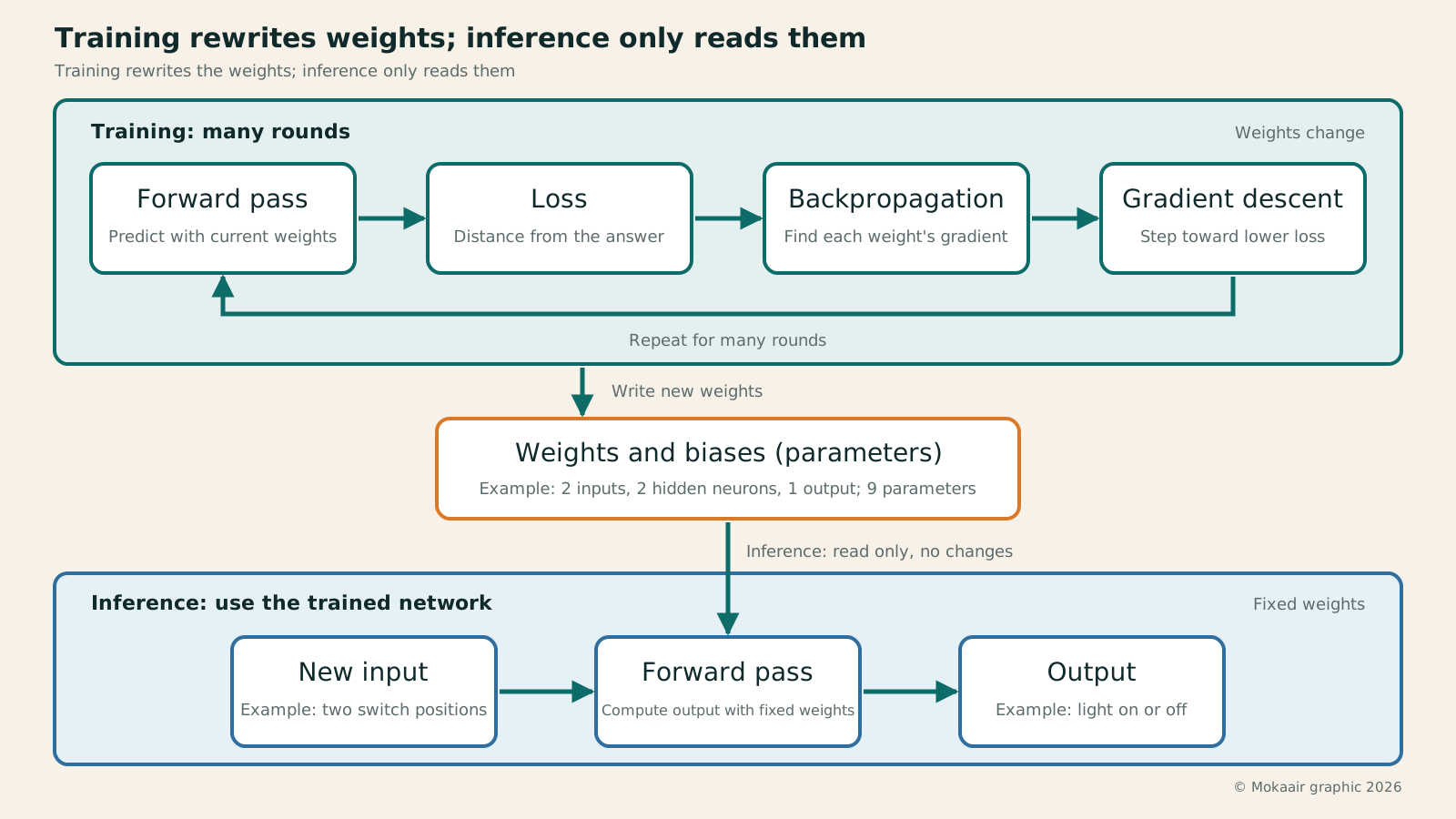
Training repeatedly performs four steps:
- Forward pass: calculate predictions using the current weights.
- Loss: measure how far predictions are from the answers. Rumelhart et al. used E = ½ ΣΣ (y − d)², summing over every output for every sample, where y is the output and d is the desired value.
- Backpropagation: apply the chain rule backward from the output to calculate how much a small change in each weight would increase or decrease the loss—the gradient. In plain language, it asks how much responsibility each weight bears for the error.
- Gradient descent: adjust weights a small step in the direction opposite to the gradient. The learning rate determines the step size; it is a hyperparameter set by a person.
Continuing the example (calculated by hand), keep the hidden layer unchanged and suppose the output-layer weights are not yet right: they are 1 and −1.2, with bias 0. For input (1,1), the hidden values are 2 and 1, the output is 0.8, the target is 0 and the loss is 0.32. The rate of change of loss with respect to the output is 0.8. Multiplying this by the respective hidden values gives weight gradients of 1.6 and 0.8; the bias gradient is 0.8. To keep the arithmetic simple, this step updates only the output layer. With a learning rate of 0.1, the weights become 0.84 and −1.28, the bias becomes −0.08 and the output falls to 0.32. In actual training, hidden-layer weights are updated in the same step too: multiply the error by the output weights, check whether ReLU is active and propagate backward all the way. That is the “back” in backpropagation. Updating the hidden layer as well would produce different numbers from those shown here.
But this step also affects other inputs: (0,1) originally produced 1, but after updating only the output layer it produces 0.76. All inputs share the weights, so changing them for one sample affects others. We therefore need to consider the average gradient across a batch of samples and repeat small steps over many rounds. Stochastic gradient descent, as described by LeCun et al., estimates the gradient using only a small batch of samples at each step.
Once training is complete, the weights are fixed. During use, the network only runs a forward pass, without calculating loss or changing weights. Google's glossary says training determines the weights, while inferenceWhat Is Inference? The Computation Behind Every Response After Model TrainingInference uses a trained model to process new inputs and produce outputs, with weights fixed throughout. This article breaks language model inference into prefill and decode, explains the differences between time to first token, end-to-end latency and throughput, distinguishes inference from reasoning and cloud from local execution, and shows what batching, quantization and caching each save.Read the full article uses the learned weights to make predictions. Any later update to the weights is a separate round of training.
Read the full description
At the top is training: four steps—forward pass, loss, backpropagation and gradient descent—repeat, with each round writing new weights into the weights and biases in the middle. The example is a small network with two inputs, two hidden neurons and one output, totaling nine parameters. At the bottom is inference: new inputs arrive, and the forward pass only reads the fixed weights to produce outputs, without calculating loss or changing weights.
Parameters, Neurons and Capability Are Three Different Things
The example has only 3 computational units but 9 parameters: each hidden neuron has 2 weights plus 1 bias, and the output unit also has 2 plus 1. Increasing the hidden layer to 100 neurons would give 100 × (2 + 1) + (100 + 1) = 401 parameters. Google's glossary defines parameters as weights and biases learned during training, whereas the learning rate is a hyperparameter supplied by a person. See model parametersWhat Are Model Parameters?Model parameters are values adjusted during training to map inputs to outputs, such as weights and biases. Simple equations show how they affect predictions and distinguish them from training hyperparameters, prompts and generation settings. Learn why parameter count, numerical precision and active parameters are different metrics, how to read model specs, why more parameters do not mean more individual facts, and why each chat does not mean retraining the model.Read the full article.
More parameters do not necessarily mean greater capability; architecture, training data and loss design also matter. LeCun et al.'s review reminds us that model quality depends on performance on test data unseen during training—in other words, generalization. Cybenko's result likewise says only that a sufficiently large network can represent a function, without guaranteeing that training can find it. When you see neuron counts, parameter counts or layer counts, ask how the model performs on your task with unseen data.
| Term | In the Example | Common Misconception |
|---|---|---|
| Neuron | A computational unit | Equivalent to a biological nerve cell |
| Weights and biases | 9 numbers to learn | Rules written by hand |
| Activation function | ReLU after the hidden layer | Optional |
| Learning rate | 0.1, set by a person | Learned by the network itself |
How Neural Networks Relate to Deep Learning and Transformer
Google's glossary calls a neural network with more than one hidden layer a deep model. LeCun et al. define deep learning as an approach that stacks multiple simple nonlinear modules and learns representations at each layer from data. Put simply, a neural network is the structure, and deep learningWhat Is Deep Learning?Deep learning uses multilayer neural networks to learn representations at different levels, often for image, speech and text tasks. Classifying recyclables in photos illustrates hidden layers, nonlinearity, training and inference, why models may memorize backgrounds rather than objects, and trade-offs in data, compute and interpretability. Learn its relation to machine learning and use new shooting conditions to check whether a model has learned useful patterns.Read the full article is the practice of learning representations through a multilayer structure. Definitions differ slightly: Google's glossary defines a neural network as a model with “at least one hidden layer,” which excludes models that connect inputs directly to outputs. Rumelhart et al., meanwhile, considered the original perceptron's intermediate layer to lack true hidden units because its connections were fixed. This article's opening definition does not use hidden layers as the dividing line. When reading, first check which definition the author is using.
Transformer is one way to arrange a network. Vaswani et al. (2017) described it as a network architecture based entirely on attention mechanisms. Alongside self-attention, each layer contains a feedforward network consisting of two linear transformations with a ReLU between them—the weighted summation plus nonlinearity described earlier. Whether later language models use this design, and how they modify it, requires checking their respective technical documentation. Neural networks are therefore the broader category. Chatbots are just one use; a small network that classifies photos belongs to the category too.
To explore other terms, start with the AI Terms Index.
Found this guide helpful? Share it with someone who needs it
Lifestyle
Agentic Retrieval-Augmented Generation (Agentic RAG): When to Search Again
Agentic RAG lets models make retrieval decisions, choosing sources, rewriting queries or searching further based on the question and available evidence. Using a concrete LangGraph workflow and a comparison of venue-use conditions, this article contrasts it with fixed RAG and explains stopping criteria, permissions, query logs and cost control. Learn to judge whether a task needs dynamic exploration or a predictable fixed workflow is enough.
Lifestyle
Graph Retrieval-Augmented Generation (GraphRAG): Understanding a Document Collection Through Relationships
GraphRAG uses entities and relationships in retrieval to answer questions about cross-document connections and overall themes. Drawing on Microsoft's original paper and official docs, this article explains entity extraction, community summaries, and local and global search, using local event records to show why different questions need different paths. It also shows how missing links, mistaken name merges, and distorted summaries affect answers: a pretty graph is not verified fact.
Lifestyle
Knowledge Graphs: Making Entities and Relationships Clear
Knowledge graphs organize entities and relationships to trace who took part in what, where and when through links. Using community events, this article covers entity identity, relationship direction, sources and time; compares Resource Description Framework (RDF) and property graphs; and explains why graphs are not equivalent to visualizations or reliable facts. Learn when to build one and how it works with tables, vector search and graph retrieval-augmented generation (GraphRAG).
Lifestyle
Hybrid Search: Balancing Exact Terms and Meaning
Hybrid search merges full-text, vector and other retrieval results to cover exact codes and natural-language needs. An equipment-manual query explains candidate retrieval, deduplication, rank fusion and reranking, including how Reciprocal Rank Fusion (RRF) merges results by rank. Hybrid search is not always more accurate. Learn to test quality with code, paraphrase and no-answer queries and spot biases from permissions, filters and duplicate content.
Articles that cite this one
Sources
- Rosenblatt 1958: The Perceptron (Psychological Review 65(6), original perceptron paper)Checked:
- Rumelhart, Hinton, Williams 1986: Learning representations by back-propagating errors (Nature 323)Checked:
- LeCun, Bengio, Hinton 2015: Deep learning (Nature 521)Checked:
- Cybenko 1989: Approximation by superpositions of a sigmoidal function (Math. Control Signals Systems 2)Checked:
- Vaswani et al. 2017: Attention Is All You Need (arXiv:1706.03762, original Transformer paper)Checked:
- Google Machine Learning Crash Course: Neural networks (unit overview)Checked:
- Google Machine Learning Crash Course: Nodes and hidden layersChecked:
- Google Machine Learning Crash Course: Activation functionsChecked:
- Google Machine Learning Crash Course: Training using backpropagationChecked:
- Google Machine Learning Glossary (entries including neural network, neuron, weight, parameter and backpropagation)Checked:
Compiled from the references and verification dates listed above; fares, schedules, product features, and terms can change, so please confirm the latest details on the relevant official website before travelling, booking, or purchasing.